Econometrics I
TA Christian Alemán
Session 2: Tuesday 1st, February 2022
Activity 1: Basic Matrix Operations
A simple structural national income model

Boring solution:
![$Y^{*} = \frac{1}{1-b}[I_{0}+G_{0}+a]$](s2_eq00238636735775643446.png)
![$C^{*} = \frac{1}{1-b}[b(I_{0}+G_{0})+a]$](s2_eq10205195815201881564.png)
Using Linear Algebra: Transform to  form
form
![$A = \left[\begin{array}{cc}1 & 0 \\ 0 & a \end{array}\right]$](s2_eq07288002101229768351.png) ,
, ![$x = \left[\begin{array}{c}Y \\ C \end{array}\right]$](s2_eq10061357105286525760.png) ,
, ![$d = \left[\begin{array}{c}I_{0}+G_{0} \\ a \end{array}\right]$](s2_eq13145882043246743807.png)

% Housekeeping
clear all
close all
clc
%
par.b = 0.5;    % Propensity to consume
par.a = 1;      % Basic Consumption
par.I = 0;      % Investment
par.G = 0.2;    % Goverment Spending
A_mat = [1,-1;-par.b,1];
d_vec = [par.I+par.G; par.a];

% Boring Solution:
Y_an = 1/(1-par.b).*(par.I+par.G+par.a);
C_an = 1/(1-par.b).*(par.b*(par.I+par.G)+par.a);
disp([])
opt.v_names = {'Y','C'};
c_table = array2table([Y_an,C_an],'VariableNames',opt.v_names);
disp('Boring Solution')
disp('')
disp(c_table)

% Using Linear Algebra:
x = inv(A_mat)*d_vec;
x = A_mat\d_vec;
c_table = array2table(x','VariableNames',opt.v_names);
disp('Solution with linear algebra')
disp('')
disp(c_table)
Boring Solution
     Y      C
    ___    ___

    2.4    2.2

Solution with linear algebra
     Y      C
    ___    ___

    2.4    2.2
Activity 2: Inverses and their properties
Define the inverse of matrix  as
as 
Such that 
-The inverse is a derived matrix that may not exist.
-The inverse of a matrix is defined if:
- is a square matrix and
- is is said to be nonsingular. Non-singularity:
 squareness and linear independence
- More in Non-Singularity:
- A singular matrix has determinant equal to zero
- A nonsingular matrix hasa non-zero determinant.
2.1 Linear independence
Let be matrix 
and  a column vector
  collecting the
  row vectors in
Linear independence requiers that the only set of scalars  which can satisfy:

are  for all
Example 1:
![$X = \left[\begin{array}{ccc}3 & 4& 5 \\ 0 & 1&2 \\ 6&8&10\end{array}\right] = \left[\begin{array}{c}v_{1}\\v_{2}\\v_{3}\end{array}\right]$](s2_eq02143686478653965004.png)
the rows are not linearly independent because 
(i.e) ![$\lambda = [2;0;-1]$](s2_eq01173836379530996867.png)
% A Singular Matrix:

X_mat = [3,4,5;0,1,2;6,8,10];

X_mat(3,:)-2.*X_mat(1,:)
ans =

     0     0     0
A non-singular matrix:
Y_mat = magic(3);
2.2 Eigenvalues and Determinants

Let the  value that solves the above system of equations be called an eigenvector
and  be the respective eigen value
Define the trace of a Matrix as:
Define the determinant of a Matrix as:
Example 2:
% Using Matlab In-built
disp('Using Matlab In-Built')
disp([det(X_mat),det(Y_mat)])

% Using our function
disp('Using Our Function')
disp([my_det(X_mat),my_det(Y_mat)])
Using Matlab In-Built
     0  -360

Using Our Function
         0 -360.0000
2.3 The rank of a matrix
The (row) rank of a matrix is defined to be the maximum number of linearly independent rows.
i.e the rank of a matrix is the number of non-zero row in the row-echelon form of the matrix.
Redefining Conditions for the existence of an inverse
The inverse of a squaren matrix exists if and only if it is of full rank.
Example 3:
% Use matlab in-built function
disp('Using Matlab In-Built')
disp([rank(X_mat),rank(Y_mat)])

% Use our function
disp('Using Our Function')
disp([my_rank(X_mat),my_rank(Y_mat)])
Using Matlab In-Built
     2     3

Using Our Function
     2     3
2.4 The inverse of a Matrix (if it exists)
Use matlab in-built function
disp(inv(Y_mat))
disp(my_inv(Y_mat))
    0.1472   -0.1444    0.0639
   -0.0611    0.0222    0.1056
   -0.0194    0.1889   -0.1028
Use our function
disp(my_inv(Y_mat))
    0.1472   -0.1444    0.0639
   -0.0611    0.0222    0.1056
   -0.0194    0.1889   -0.1028
2.5 Symetric and Idempotent Matrices
2.5.1 Symetry
A square matrix that satisfies the property  is said to be symmetric.
2.5.2 Idempotent
A square matrix is idempotent if 
If the matrix is symetric it follows that 
Idempotent matrices have that 
Idempotent matrices are very important in econometrics: Let be an (n,k) matrix of data of  . Then the matrix
Example 4:
The data generating process
 Where
Where 
% Number of observation
rng(4567)
par.n = 500;
% Simulate x
par.mean_x = 4;
par.variance_x = 2;
par.variance_e = 0.1;
x = par.mean_x +sqrt(par.variance_x).*randn(par.n,1);
% Simulate error
e = 0 + sqrt(par.variance_e).*randn(par.n,1);
% Simulate Data Generating Process:
par.beta0 = 2;
par.beta1 = 0.5;
y = par.beta0 + par.beta1.*x +e;

% Show that $M=X(X'X)^{-1}X'$ is idempotent
M = x*inv(x'*x)*x';
M_new = M*M;
I = (M-M_new).^2;
disp('Total Squared Diference:')
disp(sum(I,'all'))
Total Squared Diference:
   6.8891e-32
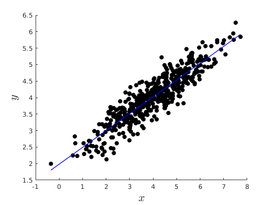
Activity 3: Least Squares Estimation:
Estimate the above model using Least Squares
Example 5:
Least Squares Estimate our function
vars = ols_esti(y,[ones(par.n,1) x]);
opt.v_names = {'\beta_{0}','\beta_{1}'};
c_table = array2table(vars.beta_hat','VariableNames',opt.v_names);
disp('OLS estimates: Our Function')
disp(c_table)


% Least Squares Estimate In-Built function
vars.beta_matlab = regress(y,[ones(par.n,1) x]);
c_table = array2table(vars.beta_matlab','VariableNames',opt.v_names);
disp('OLS estimates: In-built')
disp(c_table)

% figure
figure(1)
hold on
plot(x,y,'ko','MarkerFaceColor','k')
plot(x,vars.y_hat,'b-','linewidth',1.1)
xlabel('$x$','fontsize',17,'interpreter','latex')
ylabel('$y$','fontsize',17,'interpreter','latex')
here
OLS estimates: Our Function
    \beta_{0}    \beta_{1}
    _________    _________

     1.9818       0.51008

OLS estimates: In-built
    \beta_{0}    \beta_{1}
    _________    _________

     1.9818       0.51008
Activity 4: Using the Symbolic toolbox to do stuff
In this case to find the inverse of a matrix
My take(purely personal): AVOID using symbolic stuff, not helpfull at all.
syms a11 a12 a13 b21 b22 b23 c31 c32 c33
A_m = [a11,a12,a13;b21,b22,b23;c31,c32,c33];
A_inv = inv(A_m);
disp(A_inv)

syms a
A_m = [sym(1),sym(0),sym(0);sym(0),sym(1),sym(0);sym(0),sym(0),a];
A_inv = inv(A_m);
disp(A_inv)
[ (b22*c33 - b23*c32)/(a11*b22*c33 - a11*b23*c32 - a12*b21*c33 + a12*b23*c31 + a13*b21*c32 - a13*b22*c31), -(a12*c33 - a13*c32)/(a11*b22*c33 - a11*b23*c32 - a12*b21*c33 + a12*b23*c31 + a13*b21*c32 - a13*b22*c31),  (a12*b23 - a13*b22)/(a11*b22*c33 - a11*b23*c32 - a12*b21*c33 + a12*b23*c31 + a13*b21*c32 - a13*b22*c31)]
[-(b21*c33 - b23*c31)/(a11*b22*c33 - a11*b23*c32 - a12*b21*c33 + a12*b23*c31 + a13*b21*c32 - a13*b22*c31),  (a11*c33 - a13*c31)/(a11*b22*c33 - a11*b23*c32 - a12*b21*c33 + a12*b23*c31 + a13*b21*c32 - a13*b22*c31), -(a11*b23 - a13*b21)/(a11*b22*c33 - a11*b23*c32 - a12*b21*c33 + a12*b23*c31 + a13*b21*c32 - a13*b22*c31)]
[ (b21*c32 - b22*c31)/(a11*b22*c33 - a11*b23*c32 - a12*b21*c33 + a12*b23*c31 + a13*b21*c32 - a13*b22*c31), -(a11*c32 - a12*c31)/(a11*b22*c33 - a11*b23*c32 - a12*b21*c33 + a12*b23*c31 + a13*b21*c32 - a13*b22*c31),  (a11*b22 - a12*b21)/(a11*b22*c33 - a11*b23*c32 - a12*b21*c33 + a12*b23*c31 + a13*b21*c32 - a13*b22*c31)]

[1, 0,   0]
[0, 1,   0]
[0, 0, 1/a]
%-------------------------------------------------------------------------
% Adjoint Function
function AD = my_adjoint(X)
%{
This function computes the adjoint matrix of a square matrix
Input:
X: Square matrix
Output:
D: adjoint of the matrix X
%}
[N,M] = size(X);
if N~=M
    error('Input matrix not a square matrix.')
end
C = NaN(N,N);
for ki=1:N
   for kj = 1:N
      % Compute the cofactor matrix
      C(ki,kj) = (-1)^(ki+kj)*det(X([1:ki-1 ki+1:N],[1:kj-1 kj+1:N]));
   end
end
AD = C';
end
%-------------------------------------------------------------------------
% Inverse function
function [inv_mat] = my_inv(X)
%{
This function computes the Inverse of a square matrix if it exists
Input:
X: Square matrix
Output:
inv_mat: Inverse of the matrix X
%}
[N,M] = size(X);
if N~=M
    error('Input matrix not a square matrix.')
end
if rank(X)~=N
    error('Input matrix not full rank.')
end
inv_mat = (1/det(X)).*my_adjoint(X);
end
%-------------------------------------------------------------------------
% Determinant function
function [D] = my_det(X)
%{
This function computes the Determinant of a square matrix
Input:
X: Square matrix
Output:
D: determinant of the matrix X
%}
[N,M] = size(X);
if N~=M
    error('Input matrix not a square matrix.')
end
eig_val = eig(X); % Eigen values
D = prod(eig_val);
if abs(D)<1e-13
    D = 0;
end
end
%-------------------------------------------------------------------------
% Rank function
function [rank] = my_rank(X)
%{
This function computes the rank of a square matrix
Input:
X: Square matrix
Output:
rank: rank of the matrix X
%}
[N,M] = size(X);
if N~=M
    error('Input matrix not a square matrix.')
end
ech_mat = rref(X); % Echelon reduction
sum_ech_mat = sum(abs(ech_mat),2);
I = sum_ech_mat==0;
rank = N - sum(I);
end
%-------------------------------------------------------------------------
% OLS
function [vars] = ols_esti(y,X)
%{
This function computes the Least Squares Estimate
Input:
y: Dependent Variable    (N,1)
X: Independent Variables (N,K)
Output:
Many stuff you saw in class.

%}
[par.Nx,par.K] 	= size(X);   % N=no.obs; K=no.regressors
[par.Ny] 	= size(y,1); %

if par.Ny~=par.Nx
    error('X and y do not have same length')
end
par.N = par.Nx; % Save number of regressots

vars.beta_hat  = X\y;
% Coefficients:
vars.beta_hat_alt  = inv(X'*X)*(X'*y);
% Predicted values:
vars.y_hat 	= X*vars.beta_hat;
% Residuals:
vars.e_hat 	= y-X*vars.beta_hat;
% Total Variation of the dependent variable
vars.SST 	= (y - mean(y))'*(y - mean(y));
% (SSE) Sum Squared Residuals
vars.SSE	= vars.e_hat'*vars.e_hat;
% SSR/SST or "r-squared" is the ratio of the variation in y explained by the model and the total variation of y
vars.R2 	= 1 - (vars.SSE/vars.SST);
% Adjusted "r-squared".
vars.R2A 	= 1 - (vars.SSE/(par.N-par.K))/(vars.SST/(par.N-1));

vars.sigma2_hat = vars.SSE/(par.N-par.K);

%Variance of estimator:
vars.var_covar  = vars.sigma2_hat*inv(X'*X);
vars.SEbeta_hat = sqrt(diag(vars.var_covar));
disp('here')
end
    0.1472   -0.1444    0.0639
   -0.0611    0.0222    0.1056
   -0.0194    0.1889   -0.1028