Econometrics I

TA Christian Alemán

Session 4: Friday 11, February 2022

Based on Prof.Michael Creel's Lecture Notes And Fumio Ayashi's Book Econometrics section 1.7

Activity 1: "Replicating Nerlove"

Nerlove’s 1963 paper is a classic study of returns to scale in a regulated industry.

Firms Minimize Cost:

$C = p_{l}l+p_{f}f+p_{k}k$

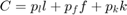
Subject to a Constant Returns to Scale Production Function (Cobb-Douglas)

$Q = F\,l^{\alpha_{1}}\,f^{\alpha_{2}}\,k^{\alpha_{3}}$

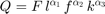
Where $l,f,k$ are the inputs, labor, fuel and capital respectively.

Equilibirum prices are respectively $p_{l},p_{f},p_{k}$ .

Recall that we have constant returns to scale if:

$\sum_{i}\alpha_{i} = r = 1$

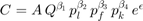
Solving the minization problem we find that the Cost Function is also Cobb-Douglas:

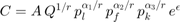
$C = A\,Q^{1/r}\,p_{l}^{\alpha_{1}/r}\,p_{f}^{\alpha_{2}/r}\,p_{k}^{\alpha_{3}/r}\,e^{\epsilon}$

Whats more, the cost function above will be homogeneous of degree 1 (HOD1) if $\sum_{i}=\alpha_{i}/r = 1$

We can rewrite the above cost function as:

$C = A\,Q^{\beta_{1}}\,p_{l}^{\beta_{2}}\,p_{f}^{\beta_{3}}\,p_{k}^{\beta_{4}}\,e^{\epsilon}$

Take the logs

$ln(C) = \beta_{1} +\beta_{2}ln(Q)+\beta_{3}ln(p_{l})+\beta_{4}ln(p_{f})+\beta_{5}ln(p_{l})+ \epsilon$

Our Data

Data on Company's:

COST(C)
OUTPUT(Q)
PRICE OFLABOR $(p_{L})$
PRICE OF FUEL $(p_{f})$
PRICE OF CAPITAL $(p_{K})$ .

We are ready to run some tests!

We want to test:

Constant Returns to Scale (CRS) assumption
Homogeneity of degree 1
Understant whether CRS changes with size of the company

Our Tools:

Restricted estimation:
Testing: Chow-test

% Housekeeping
clc
close all
clear all

% Load the Data
load nerlove

data = data(:,2:6);
data = log(data);
n = size(data,1);
y = data(:,1);
x = data(:,2:5);
x = [ones(n,1), x];
k = size(x,2);

names = str2mat("constant", "output","labor", "fuel", "capital");
names = [names; names; names; names; names]; % copy 5 times for Chow test
% Run OLS
[b,~,~,~] = mc_ols(y,x,names, 0, 1);

*********************************************************
OLS estimation results
Observations 145
R-squared 0.925955
Sigma-squared 0.153943

Results (Ordinary var-cov estimator)

   estimate   st.err.   t-stat.   p-value  
1      -3.527       1.774      -1.987       0.049
2       0.720       0.017      41.244       0.000
3       0.436       0.291       1.499       0.136
4       0.427       0.100       4.249       0.000
5      -0.220       0.339      -0.648       0.518

*********************************************************

Activity 2: Testing

Testing Homogeneity of Degree 1

Recall the linear restriction form:

$R\beta = r$

In our case for HOD1 we need $r=1$ and $R=(0,0,1,1,1)$

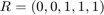
The null hypothesis for qF,Wald,LR test below is:

$H_{0}: R\beta = r$

$H_{1}: R\beta \neq r$

We cannot reject the null (the p-value is above 0.05), meaning that we cannot reject Homogeneity

% First Homogeneity of Degree 1 (HOD1)
R = [0, 0, 1, 1, 1];
r = 1;
% Imposing and testing HOD1
mc_olsr(y, x, R, r, names);
TestStatistics(y, x, R, r);

For some reason the output of this example is comming at the end of the page.

Testing Constant Returns to scale (CRS)

In our case for CRS we need 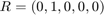$r=1$ and $R=(0,1,0,0,0)$

$H_{0}: R\beta = r$

$H_{1}: R\beta \neq r$

We reject the null (the p-value is below 0.05), meaning that we reject the assumption of constant returns to scale.

% Now Constant Returs to Scale (CRTS)
R = [0, 1, 0, 0, 0];
r = 1;
 % Imposing and testing CRTS
mc_olsr(y, x, R, r, names);
TestStatistics(y, x, R, r);

Restricted LS estimation results
Observations 145
R-squared 0.790420
Sigma-squared 0.438861

Results (Het. consistent var-cov estimator)

   estimate   st.err.   t-stat.   p-value  
1      -7.530       2.919      -2.579       0.011
2       1.000       0.000         Inf       0.000
3       0.020       0.376       0.052       0.959
4       0.715       0.159       4.490       0.000
5       0.076       0.576       0.132       0.896

*********************************************************
          Value   p-value  
F         256.262       0.000
Wald      265.414       0.000
LR        150.863       0.000
Score      93.771       0.000

Activity 3: The chow test

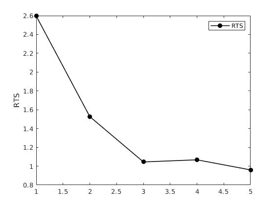
We want to understant whether CRS changes with size of the company

Define 5 subsamples of firms, with thefirst group being the 29 firms with the lowest output levels, then the next 29 firms, etc.

To do this define dummy variables:

$D_{1}=\begin{cases}1\, t\in\{1,2,...,29\}\end{cases}$ $0$ Otherwise

$D_{2}=\begin{cases}1\, t\in\{30,31,...,58\}\end{cases}$ $0$ Otherwise

And so forth fro $D_{3},...,D_{5}$

Then the model can be rewritten as:

$ln(C) = \sum_{j}^{5}D_{j}\beta_{1} +\sum_{j}^{5}D_{j}\beta_{2,j}ln(Q)+\sum_{j}^{5}D_{j}\beta_{3,j}ln(Pl)+\sum_{j}^{5}D_{j}\beta_{4,j}ln(Pf)+\sum_{j}^{5}D_{j}\beta_{5,j}ln(Pl)+ \epsilon$

In Matrix form

$\left[\begin{array}{c}y_{1} \\ y_{2} \\ y_{3} \\ y_{4} \\ y_{5} \end{array}\right]=\left[\begin{array}{ccccc}X_{1}&0&0&0&0 \\ 0&X_{2}&0&0&0 \\ 0&0&X_{3}&0&0 \\ 0&0&0&X_{4}&0 \\ 0&0&0&0&X_{5} \end{array}\right]\left[\begin{array}{c}\beta^{1} \\ \beta^{2} \\ \beta^{3} \\ \beta^{4} \\ \beta^{5} \end{array}\right]\left[\begin{array}{c}\epsilon_{1} \\ \epsilon_{2} \\ \epsilon_{3} \\ \epsilon_{4} \\ \epsilon_{5} \end{array}\right]$

We define $\beta^{j} = (\beta_{1},\beta_{2,j},\beta_{3,j},\beta_{4,j},\beta_{5,j})$

% Create the block diagonal X matrix corresponding to separate coefficients
big_x = zeros(n,5*k);
%x_A = NaN()
x_old = x;
for i=1:k
	startrow = (i-1)*29+1;
	endrow = i*29;
	startcol =(i-1)*k + 1;
	endcol = i*k;
	big_x(startrow:endrow,startcol:endcol) ...
        = big_x(startrow:endrow,startcol:endcol)...
		+ x(startrow:endrow,:);
    % Alternative X
%    x_A(:,:,i) = x(startrow:endrow,:);
end
x = big_x;

Visual Inspection

Nerlove model: 5 separate regressions, one per each group of firms

b = mc_ols(y, x, names);
output = 1:5;
output = output*5+2-5; % Just extract the relevant parameter
output = b(output,:);
rts = 1 ./ output;

% gset term X11
xlabel("Output group");
group = 1:5;

figure(1)
plot(group, rts,"ko-",'linewidth',1.2,'markerfacecolor','k')
ylabel('RTS')
legend('RTS')

*********************************************************
OLS estimation results
Observations 145
R-squared 0.960901
Sigma-squared 0.094836

Results (Het. consistent var-cov estimator)

          estimate   st.err.   t-stat.   p-value  
constant       0.390       4.049       0.096       0.923
output         0.385       0.089       4.315       0.000
labor         -0.177       0.894      -0.198       0.844
fuel           0.406       0.255       1.591       0.114
capital       -0.650       0.744      -0.873       0.384
constant      -0.569       1.937      -0.294       0.769
output         0.655       0.077       8.490       0.000
labor         -0.522       0.284      -1.834       0.069
fuel           0.511       0.090       5.669       0.000
capital       -0.681       0.375      -1.819       0.071
constant      -2.146       1.724      -1.245       0.216
output         0.957       0.135       7.095       0.000
labor         -0.335       0.208      -1.610       0.110
fuel           0.409       0.120       3.408       0.001
capital       -0.722       0.264      -2.739       0.007
constant      -4.934       1.732      -2.849       0.005
output         0.937       0.106       8.865       0.000
labor          0.313       0.238       1.313       0.192
fuel           0.439       0.061       7.206       0.000
capital       -0.255       0.293      -0.871       0.386
constant      -6.946       1.828      -3.800       0.000
output         1.041       0.064      16.339       0.000
labor          0.642       0.228       2.818       0.006
fuel           0.679       0.097       7.039       0.000
capital       -0.239       0.288      -0.830       0.408

*********************************************************

Chow test

When performing the Chow Tets the null to test is that the parameter vectors for the separate groups are all the same, that is:

$H_{0}: \beta^{1}=\beta^{2}=...=\beta^{5}$

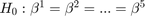
We reject the null, then the estimated coefficients are different for the 5 groups.

R = eye(5);
Z = zeros(5,5);
R = [
	R -R Z Z Z;
	R Z -R Z Z;
	R Z Z -R Z;
	R Z Z Z -R
	];
r = zeros(20,1);

% Chow test:
mc_olsr(y, x, R, r, names);
TestStatistics(y, x, R, r);

Restricted LS estimation results
Observations 145
R-squared 0.925955
Sigma-squared 0.215520

Results (Het. consistent var-cov estimator)

          estimate   st.err.   t-stat.   p-value  
constant      -3.527       1.689      -2.088       0.039
output         0.720       0.032      22.491       0.000
labor          0.436       0.241       1.808       0.074
fuel           0.427       0.074       5.751       0.000
capital       -0.220       0.318      -0.691       0.491
constant      -3.527       1.689      -2.088       0.039
output         0.720       0.032      22.491       0.000
labor          0.436       0.241       1.808       0.074
fuel           0.427       0.074       5.751       0.000
capital       -0.220       0.318      -0.691       0.491
constant      -3.527       1.689      -2.088       0.039
output         0.720       0.032      22.491       0.000
labor          0.436       0.241       1.808       0.074
fuel           0.427       0.074       5.751       0.000
capital       -0.220       0.318      -0.691       0.491
constant      -3.527       1.689      -2.088       0.039
output         0.720       0.032      22.491       0.000
labor          0.436       0.241       1.808       0.074
fuel           0.427       0.074       5.751       0.000
capital       -0.220       0.318      -0.691       0.491
constant      -3.527       1.689      -2.088       0.039
output         0.720       0.032      22.491       0.000
labor          0.436       0.241       1.808       0.074
fuel           0.427       0.074       5.751       0.000
capital       -0.220       0.318      -0.691       0.491

*********************************************************
          Value   p-value  
F           5.363       0.000
Wald      129.601       0.000
LR         92.595       0.000
Score      68.434       0.000

Pick another reference, results should be the same

Chow test: note that the restricted model gives the same results as the original model

R = eye(5);
Z = zeros(5,5);
R = [
	-R Z Z Z R;
	Z -R Z R Z;
	Z Z -R Z R;
	-R R Z Z Z
	];
r = zeros(20,1);

mc_olsr(y, x, R, r, names);
TestStatistics(y, x, R, r);

Restricted LS estimation results
Observations 145
R-squared 0.925955
Sigma-squared 0.215520

Results (Het. consistent var-cov estimator)

          estimate   st.err.   t-stat.   p-value  
constant      -3.527       1.689      -2.088       0.039
output         0.720       0.032      22.491       0.000
labor          0.436       0.241       1.808       0.074
fuel           0.427       0.074       5.751       0.000
capital       -0.220       0.318      -0.691       0.491
constant      -3.527       1.689      -2.088       0.039
output         0.720       0.032      22.491       0.000
labor          0.436       0.241       1.808       0.074
fuel           0.427       0.074       5.751       0.000
capital       -0.220       0.318      -0.691       0.491
constant      -3.527       1.689      -2.088       0.039
output         0.720       0.032      22.491       0.000
labor          0.436       0.241       1.808       0.074
fuel           0.427       0.074       5.751       0.000
capital       -0.220       0.318      -0.691       0.491
constant      -3.527       1.689      -2.088       0.039
output         0.720       0.032      22.491       0.000
labor          0.436       0.241       1.808       0.074
fuel           0.427       0.074       5.751       0.000
capital       -0.220       0.318      -0.691       0.491
constant      -3.527       1.689      -2.088       0.039
output         0.720       0.032      22.491       0.000
labor          0.436       0.241       1.808       0.074
fuel           0.427       0.074       5.751       0.000
capital       -0.220       0.318      -0.691       0.491

*********************************************************
          Value   p-value  
F           5.363       0.000
Wald      129.601       0.000
LR         92.595       0.000
Score      68.434       0.000

Run the Chow test only the last two groups:

% Trim the data
% ng: Choose number of groups :
%

ng = 2;
ni = 5-ng;
y = y(29*ni+1:end,1);
x = x(29*ni+1:end,5*ni+1:end);


R = eye(5);
Z = zeros(5,5);

R = [R -R];
r = zeros(5*(ng-1),1);

Chow test: note that we still reject the null, but only at the 95% level, not at 90% anymore

mc_olsr(y, x, R, r, names);
TestStatistics(y, x, R, r);

Restricted LS estimation results
Observations 58
R-squared 0.961866
Sigma-squared 0.026330

Results (Het. consistent var-cov estimator)

   estimate   st.err.   t-stat.   p-value  
1      -5.526       1.437      -3.844       0.000
2       0.944       0.037      25.746       0.000
3       0.616       0.180       3.430       0.001
4       0.434       0.056       7.694       0.000
5      -0.190       0.257      -0.740       0.463
6      -5.526       1.437      -3.844       0.000
7       0.944       0.037      25.746       0.000
8       0.616       0.180       3.430       0.001
9       0.434       0.056       7.694       0.000
10      -0.190       0.257      -0.740       0.463

*********************************************************
          Value   p-value  
F           2.487       0.044
Wald       15.028       0.010
LR         13.363       0.020
Score      11.936       0.036

Display Code ends for publication

disp('code ends')

code ends

Functions

function [b, varb, e] = mc_olsr(y, x, R, r, names, silent, regularvc)
%{
Copyright (C) 2010 Michael Creel <michael.creel@uab.es>
This program is free software; you can redistribute it and/or modify
it under the terms of the GNU General Public License as published by
the Free Software Foundation

 Calculates restricted LS estimator (subject to Rb=r) using the Huber-White heteroscedastic
 consistent variance estimator.


 inputs:
 y: dep variable
 x: matrix of regressors
 R: matrix R in Rb=r
 r: vector r in Rb=r
 names (optional) names of regressors
 silent (bool) default false. controls screen output
 regularvc (bool) default false. use normal varcov estimator, instead of het consistent (default)

 outputs:
 b: estimated coefficients
 varb: estimated covariance matrix of coefficients (Huber-White by default, ordinary OLS if requested with switch)
 e: ols residuals
 ess: sum of squared residuals

%}
	if nargin < 7
        regularvc = false;
    end
	if nargin < 6
        silent = false;
    end
	k = size(x,2);
	if (nargin < 5) || (size(names,1) ~= k)
		names = 1:k;
		names = names';
	end

	[b, sigsq, e] = ols(y, x);

	xx_inv = inv(x'*x);
	n = size(x,1);
	k = size(x,2);
	q = size(R,1);

    try
	P_inv = inv(R*xx_inv*R');
    catch
        der_stop = 1;
    end
	b = b - xx_inv*R'*P_inv*(R*b-r);

	e = y-x*b;
	ess = e' * e;
	sigsq = ess/(n - k - q);

	% Ordinary or het. consistent variance estimate
	if regularvc==1
		varb = xx_inv*sigsq;
	else
		varb = HetConsistentVariance(x,e);
    end

	A = eye(k) - xx_inv*R'*P_inv*R;  %# the matrix relating b and b_r
	varb = A*varb*A';
	seb = sqrt(diag(varb));
	t = b./seb;

	tss = y - mean(y);
	tss = tss' * tss;
	rsq = 1 - ess / tss;

	labels = char('estimate', 'st.err.', 't-stat.', 'p-value');
	if silent==0
		('\n*********************************************************\n');
		fprintf('Restricted LS estimation results\n');
		fprintf('Observations %d\n',n);
		fprintf('R-squared %f\n',rsq);
		fprintf('Sigma-squared %f\n',sigsq);
		p = 2 - 2*tcdf(abs(t), n - k - q);
		results = [b, seb, t, p];
		if regularvc==1
			fprintf('\nResults (Ordinary var-cov estimator)\n\n');
		else
			fprintf('\nResults (Het. consistent var-cov estimator)\n\n');
		end
		prettyprint(results, names, labels);
		fprintf('\n*********************************************************\n');
    end
end
%
function varb = HetConsistentVariance(x, e)
	xx_inv = inv(x'*x);
	E = e .^2;
	varb = xx_inv * x'*eemult_mv(x, E) * xx_inv;
end
%}

function [F, W, LR, S] = TestStatistics(y, x, R, r)
%{
Copyright (C) 2010 Michael Creel <michael.creel@uab.es>
This program is free software; you can redistribute it and/or modify
it under the terms of the GNU General Public License as published by
the Free Software Foundation

This code calculates F, Wald, Score and Likelihood Ratio tests for
linear model y=XB+e e~N(0,sig^2*I_n) subject to linear restrictions RB=r

The null is H_{0}:RB=r
inputs:
 		 y: nx1 dependent variable
 		 x: nxk regressor matrix
 		 R: R above, a qxk matrix
 		 r: r above, a qx1 vector

output:  F: the F statistic
 		 W: the Wald statistic
 		 S: the score statistic
 		 LR: the likelihood ratio statistic


%}
    n = size(x,1);
    k = size(x,2);
    q = size(R,1);

    % OLS
	[b, ~, ~] = ols(y, x);

	% The restricted estimator
	xx_inv = inv(x'*x);
	P_inv = inv(R*xx_inv*R');
	b_r = b - xx_inv*R'*P_inv*(R*b-r);

  % Sums of squared errors and estimators of sig^2
  e = y - x*b;
  ess = e'*e;
  e_r = y - x*b_r;
  ess_r = e_r' * e_r;
  sigsqhat_ols = ess/(n-k);
  sigsqhat_mle = ess/(n);
  sigsqhat_mle_r = ess_r/(n);

  % F-test
  F = (ess_r-ess)/q;
  F = F/sigsqhat_ols;

  % Wald test (uses unrestricted model's est. of sig^2
  W = (R*b-r)'*P_inv*(R*b-r)/sigsqhat_mle;

  % Score test (uses restricted model's est. of sig^2
  P_x = x * xx_inv * x';
  S = e_r' * P_x * e_r/(sigsqhat_mle_r);

  % LR test
  lnl = -n/2*log(2*pi) - n/2*log(sigsqhat_mle) - e' * e/(2*sigsqhat_mle);
  lnl_r = -n/2*log(2*pi) - n/2*log(sigsqhat_mle_r) - e_r' * e_r/(2*sigsqhat_mle_r);
  LR = 2*(lnl-lnl_r);
	tests = [F;W;LR;S];
	WLRS = [W;LR;S];
	pvalues = [1 - fcdf(F,q,n-k); 1 - chi2cdf(WLRS,q)];
	tests = [tests, pvalues];

	TESTS = str2mat("F","Wald","LR","Score");
	labels = str2mat("Value","p-value ");
	prettyprint(tests, TESTS, labels);
end

function [beta,sigma,r]= ols(y,x)
% Simple OLS regression
t = size(x,1);
beta = inv (x'*x) * x' * y;
sigma = (y-x*beta)'*(y-x*beta)/(t-rank(x));
r = y - x*beta;

end

function prettyprint(mat, rlabels, clabels)
%{
This function prints matrices with row and column labels

Copyright (C) 2010 Michael Creel <michael.creel@uab.es>
This program is free software; you can redistribute it and/or modify
it under the terms of the GNU General Public License as published by
the Free Software Foundation
%}
	% left pad the column labels
	a = size(rlabels,2);
	for i = 1:a
		fprintf(' ');
	end
	fprintf('  ');

	% print the column labels
    try
	clabels = ['        ';clabels]; % pad to 8 characters wide
    catch
        dert_stop = 1;
    end
	clabels = strjust(clabels,'right');

	k = size(mat,2);
	for i = 1:k
		fprintf('%s  ',clabels(i+1,:));
	end

	% now print the row labels and rows
	fprintf('\n');
	k = size(mat,1);
	for i = 1:k
		if ischar(rlabels(i,:))
			fprintf(rlabels(i,:));
		else
			fprintf('%i', rlabels(i,:));
		end
		fprintf('  %10.3f', mat(i,:));
		fprintf('\n');
	end
end


function result = eemult_mv(m,v)

	if not(ismatrix(m))
		error("eemult_mv: first arg must be a matrix");
    end

	if not(isvector(v))
		error("eemult_mv: second arg must be a vector");
    end

	[rm, cm] = size(m);
	[rv, cv] = size(v);

	if (rm == rv)
		v = kron(v, ones(1,cm));
		result = m .* v;
	elseif (cm == cv)
		v = kron(v, ones(rm, 1));
		result = m .* v;
	else
		error("eemult_mv: dimension of vector must match one of the dimensions of the matrix");
    end
end

function [b, varb, e, ess] = mc_ols(y, x, names, silent, regularvc)
%{

Copyright (C) 2010 Michael Creel <michael.creel@uab.es>
This program is free software; you can redistribute it and/or modify
it under the terms of the GNU General Public License as published by
the Free Software Foundation

Calculates ordinary LS estimator using the Huber-White heteroscedastic
consistent variance estimator.

 inputs:
 y: dep variable
 x: matrix of regressors
 names (optional) names of regressors
 silent (bool) default false. controls screen output
 regularvc (bool) default false. use normal varcov estimator, instead of het consistent (default)

 outputs:
 b: estimated coefficients
 varb: estimated covariance matrix of coefficients (Huber-White by default, ordinary OLS if requested with switch)
 e: ols residuals
 ess: sum of squared residuals

%}
	k = size(x,2);

	if nargin < 5 regularvc = 0; end
	if nargin < 4 silent = 0; end
	if (nargin < 3) || (size(names,1) ~= k)
		names = 1:k;
		names = names';
	end

	[b, sigsq, e] = ols(y,x);

	xx_inv = inv(x'*x);
	n = size(x,1);

	ess = e' * e;

	% Ordinary or het. consistent variance estimate
	if regularvc==1
		varb = xx_inv*sigsq;
	else
		varb = HetConsistentVariance(x,e);
    end

	seb = sqrt(diag(varb));
	t = b ./ seb;

	tss = y - mean(y);
	tss = tss' * tss;
	rsq = 1 - ess / tss;

	labels = char('estimate', 'st.err.', 't-stat.', 'p-value');
	if silent==0
		fprintf('\n*********************************************************\n');
		fprintf('OLS estimation results\n');
		fprintf('Observations %d\n',n);
		fprintf('R-squared %f\n',rsq);
		fprintf('Sigma-squared %f\n',sigsq);
		p = 2 - 2*tcdf(abs(t), n - k);
		results = [b, seb, t, p];
		if regularvc
			fprintf('\nResults (Ordinary var-cov estimator)\n\n');
		else
			fprintf('\nResults (Het. consistent var-cov estimator)\n\n');
		end
		prettyprint(results, names, labels);
		fprintf('\n*********************************************************\n');
	end

end

Restricted LS estimation results
Observations 145
R-squared 0.925652
Sigma-squared 0.155686

Results (Het. consistent var-cov estimator)

   estimate   st.err.   t-stat.   p-value  
1      -4.691       0.804      -5.838       0.000
2       0.721       0.032      22.516       0.000
3       0.593       0.167       3.556       0.001
4       0.414       0.072       5.768       0.000
5      -0.007       0.154      -0.048       0.962

*********************************************************
          Value   p-value  
F           0.574       0.450
Wald        0.594       0.441
LR          0.593       0.441
Score       0.592       0.442