Econometrics I
TA Christian Alemán
Session 5: Friday 18, February 2022
Activity 1: Simulating Consistency of OLS
Consider the model
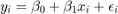
![$x\sim U[a,b]$](s5_eq07474211892256132982.png)
We will show consistency of 

Lets assume different distributions of 
- Normal :

- Poisson:

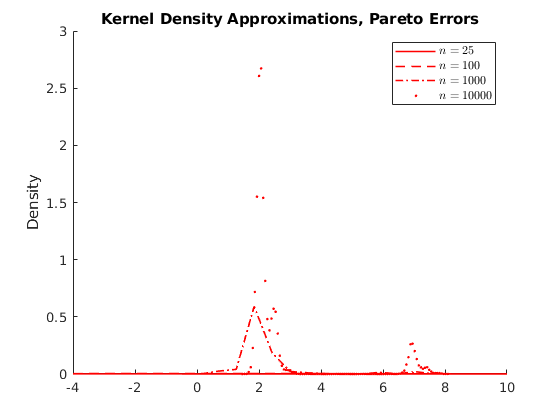
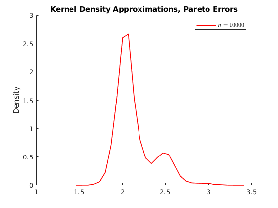
- Pareto:
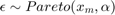
We will Simulate a population of 50000
Make 10000 draws of sample of n = [25,100,1000,10000];
% Housekeeping
clc
close all
clear all

% Set seed for reproductibility


% Options
opt.load_betas = 1;                 % 1:load betas to save time


% Parameters
par.N = 100000;                      % Population
par.n_ms = 10000;                    % Number of MC simulations
par.n_grid = [25,100,1000,10000];   % Sample size
par.beta0 = 1;
par.beta1 = 2;

% Parameters distributions of \epsilon:
par.sigma = 1;      % Standard deviation normal
par.lambda = 1;     % Poisson Rate
par.k = 1;          % Shape if >=1 var is infinity try 4
par.sigma_gp = 2;   % Scale
par.theta = 0;
par.ub = 100;
par.lb = 0;

% Generate population
vars.e_pop = NaN(par.N,3);
for i = 1:3
    if i == 1
        rng(123+i)
        vars.e_pop(:,1) = par.sigma.*randn(par.N,1);
        vars.e_pop(:,1) = vars.e_pop(:,1)-mean(vars.e_pop(:,1)); % demean
    elseif i == 2
        rng(123+i)
        vars.e_pop(:,2) = sim_poisson(par.N,par.lambda);
        vars.e_pop(:,2) = vars.e_pop(:,2)-mean(vars.e_pop(:,2));
    elseif i == 3
        rng(123+i)
        vars.e_pop(:,3) = gprnd(par.k,par.sigma_gp,par.theta,par.N,1);
        %vars.e_pop(:,3) = sim_gp(par.N,par.k,par.sigma_gp,par.theta);
        vars.e_pop(:,3) = vars.e_pop(:,3)-mean(vars.e_pop(:,3));
    end
end

vars.x_pop = unifrnd(par.lb,par.ub,par.N,1);
vars.y_pop = par.beta0 +par.beta1.*repmat(vars.x_pop,1,3) +vars.e_pop;

% Here we do the sampling and compute the distributions of parameters

% Initialize holder
vars.hbeta1 = NaN(par.n_ms,4,3);

if opt.load_betas ==1
    load('data')
    vars.hbeta1 = mc_data;
else
    % Generate NS number of samples from the universe.
    for i = 1:3  %  Distributions
        for ii = 1:4    % Sample sizes
            disp([i,ii])
            for j = 1:par.n_ms   % Number of MC simulations

                I_sample = randsample(par.N,par.n_grid(ii));
                x_sample = vars.x_pop(I_sample);
                y_sample = vars.y_pop(I_sample,i);
                % Run regression
                X = [ones(par.n_grid(ii),1),x_sample];
                Y = y_sample;
                hat_betas = X\Y;
                % Save betas
                vars.hbeta1(j,ii,i) = hat_betas(2);
            end
        end
    end

    mc_data = vars.hbeta1;
    save('data','mc_data')
    %save('data_inc','data_income')
end

vars.kdensity = NaN(100,4,3);            % Initialize Kernel Density
par.support  = NaN(100,4,3);
 for i = 1:3  %  Distributions
        for ii = 1:4    % Sample sizes
        % Do kernel approximations to smooth histograms
        [vars.kdensity(:,ii,i),par.support(:,ii,i)] = ksdensity(vars.hbeta1(:,ii,i),'Kernel','normal');
        end
 end

figure(1)
hold on
p1 = plot(par.support(:,1,1),vars.kdensity(:,1,1),'r-','linewidth',1.2);
p2 = plot(par.support(:,2,1),vars.kdensity(:,2,1),'r--','linewidth',1.2);
p3 = plot(par.support(:,3,1),vars.kdensity(:,3,1),'r-.','linewidth',1.2);
p4 = plot(par.support(:,4,1),vars.kdensity(:,4,1),'r.','linewidth',1.2);
xlim([1.98,2.02])
legend([p1 p2 p3 p4],{'$n=25$','$n=100$','$n=1000$','$n=10000$'},'interpreter','latex')
title('Kernel Density Approximations, Normal Errors')
ylabel('Density')

figure(2)
hold on
p1 = plot(par.support(:,1,2),vars.kdensity(:,1,2),'r-','linewidth',1.2);
p2 = plot(par.support(:,2,2),vars.kdensity(:,2,2),'r--','linewidth',1.2);
p3 = plot(par.support(:,3,2),vars.kdensity(:,3,2),'r-.','linewidth',1.2);
p4 = plot(par.support(:,4,2),vars.kdensity(:,4,2),'r.','linewidth',1.2);
xlim([1.98,2.02])
legend([p1 p2 p3 p4],{'$n=25$','$n=100$','$n=1000$','$n=10000$'},'interpreter','latex')
title('Kernel Density Approximations, Poisson Errors')
ylabel('Density')

figure(3)
hold on
p1 = plot(par.support(:,1,3),vars.kdensity(:,1,3),'r-','linewidth',1.2);
p2 = plot(par.support(:,2,3),vars.kdensity(:,2,3),'r--','linewidth',1.2);
p3 = plot(par.support(:,3,3),vars.kdensity(:,3,3),'r-.','linewidth',1.2);
p4 = plot(par.support(:,4,3),vars.kdensity(:,4,3),'r.','linewidth',1.2);
xlim([-4,10])
legend([p1 p2 p3 p4],{'$n=25$','$n=100$','$n=1000$','$n=10000$'},'interpreter','latex')
title('Kernel Density Approximations, Pareto Errors')
ylabel('Density')

figure(4)
hold on
p4 = plot(par.support(1:30,4,3),vars.kdensity(1:30,4,3),'r-','linewidth',1.2);
legend([p4],{'$n=10000$'},'interpreter','latex')
title('Kernel Density Approximations, Pareto Errors')
ylabel('Density')
Activity 1.1: Asymtotic Normality
Normality test for the last case H0: x comes from a standard normal distribution
name = {'Normal:','Poisson:','Pareto:'};
for i = 1:3
    disp(name{i})
    test_cdf = makedist('normal','mu',mean(vars.hbeta1(:,4,i)),'sigma',std(vars.hbeta1(:,4,i)));
    %test_cdf = [vars.hbeta1(:,4,i),cdf('normal',vars.hbeta1(:,4,i),mean(vars.hbeta1(:,4,i)),std(vars.hbeta1(:,4,i)))];
    h = kstest(vars.hbeta1(:,4,i),'CDF',test_cdf); % Test if the data are from the hypothesized distribution.
if h==1
    disp('We reject the Null: Then distribution is not normal')
else
    disp('We CANNOT reject the Null: Then distribution is normal')
end
end
Normal:
We CANNOT reject the Null: Then distribution is normal
Poisson:
We CANNOT reject the Null: Then distribution is normal
Pareto:
We reject the Null: Then distribution is not normal
Activity 2: Testing Non Linear Constrains WALD test
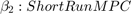
Consider the following consumption function with different short- and long-run marginal propensities to consume (MPC).

 is Consumption at
  (in real USD)
 is Disposable Income at (in real USD)
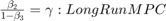
We are interested in knowing whether 
load('data_inc2')
%{
1: C0
2: C1
3: Y
%}
data_income = log(data_income);
n = size(data_income,1);
K = 3;
X = [ones(n,1),data_income(:,3),data_income(:,2)];
y = data_income(:,1);
% Compute OLS
betas = X\y;
hgamma = betas(2)/(1-betas(3));

Param = {'beta 1';'beta 2';'beta 3';'gamma'};


hat_betas = [betas;hgamma];
tab_B = table(Param,hat_betas);
disp('OLS Estimates:')
disp(tab_B)
OLS Estimates:
      Param       hat_betas
    __________    _________

    {'beta 1'}    0.0031416
    {'beta 2'}     0.074958
    {'beta 3'}      0.92462
    {'gamma' }      0.99446
Predict errors
he = y-X*betas;
hsigma = (he'*he)/(n-K);
% Compute Asymtotic VarCovar
Avar_beta = hsigma.*(inv(X'*X));
AVCV = sqrt((diag(Avar_beta)));     % Variance Covariance

% Compute the analytical derivatives:
% Derivative: \partial beta2/(1-beta3)\partial(\beta)
grad = [0;1/(1-betas(3));betas(2)/(1-betas(3))^(2)];
% Compute the asymtotic Variance
Avar_Cbeta = grad'*Avar_beta*grad;
% Since we are testing one restriction we compute the z-score:
% H0: gamma = 1
z = (hgamma-1)./sqrt(Avar_Cbeta);
disp(['Z-Score = ',num2str(z)])
disp('We cannot reject \gamma=1')
Z-Score = -0.33863
We cannot reject \gamma=1
Activity 3: Bootstrap standard errors
3.1 Non-Parametric Bootstrap
- Generate B samples with replacement of pairs

- Estimate the bootstrap
 by fitting the model
 - Compute the standard errors
par.n = par.n_grid(3);      % Sample size
par.K = 2;
vars.x =1+2*randn(par.n,2) ;
vars.x(:,1) =4+vars.x(:,1);
vars.e =2*randn(par.n,1) ;
vars.y = vars.x*ones(2 ,1) + vars.e ;
if par.K ==3
    vars.x = [ones(par.n,1),vars.x];
    vars.y = par.beta0+vars.x(:,2:end)*ones(2 ,1) + vars.e ;
end


vars.hbeta = vars.x\vars.y ;
vars.ehat = vars.y-vars.x*vars.hbeta;
par.B = 1000;%

hbeta_sample =NaN(par.B,par.K);
for i = 1:par.B

    I_sample = ceil(par.n*rand(1,par.n));
    ysample = vars.y(I_sample);
    xsample(:,1) = vars.x(I_sample,1);
    xsample(:,2) = vars.x(I_sample,2);

    hbeta_sample(i,:)  = (xsample\ysample)';
end
diff = hbeta_sample-repmat(vars.hbeta',par.B,1);
bootVCV = diff'*diff/par.B;
OLSVCV = (vars.e'*vars.e)/par.n*inv(vars.x'*vars.x);

vars.SEbeta_hat_OLS = sqrt(diag(OLSVCV));
vars.SEbeta_hat_boot = sqrt(diag(bootVCV));

Param = {'beta 0';'beta 1'};
if  par.K ==3
    Param = {'beta 0';'beta 1','beta2'};
end

SE_OLS = vars.SEbeta_hat_OLS;
SE_Bootstrap = vars.SEbeta_hat_boot;
tab_SE = table(Param,SE_OLS,SE_Bootstrap);
disp('Non-Parametric Standard Errors:')
disp(tab_SE)
Non-Parametric Standard Errors:
      Param        SE_OLS     SE_Bootstrap
    __________    ________    ____________

    {'beta 0'}    0.012984      0.012932
    {'beta 1'}    0.031073      0.030937
3.2 Parametric Bootstrap
- Generate 2*B samples with replacement of
 indepedently
 - Construct values of

- Estimate the bootstrap by fitting the model
- Compute the standard errors
for i = 1:par.B

    I_sample = ceil(par.n*rand(1,par.n));
    II_sample = ceil(par.n*rand(1,par.n));
    esample = vars.ehat(I_sample);
    xsample(:,1) = vars.x(I_sample,1);
    xsample(:,2) = vars.x(I_sample,2);
    ysample = xsample*vars.hbeta+esample;
    hbeta_sample(i,:)  = (xsample\ysample)';
end
diff = hbeta_sample-repmat(vars.hbeta',par.B,1);
bootVCV = diff'*diff/par.B;
OLSVCV = (vars.e'*vars.e)/par.n*inv(vars.x'*vars.x);

vars.SEbeta_hat_OLS = sqrt(diag(OLSVCV));
vars.SEbeta_hat_boot = sqrt(diag(bootVCV));


SE_OLS = vars.SEbeta_hat_OLS;
SE_Bootstrap = vars.SEbeta_hat_boot;
tab_SE = table(Param,SE_OLS,SE_Bootstrap);
disp('Parametric Standard Errors:')
disp(tab_SE)


dert_stop = 1;
%-----------------------------------------------------------
function data = sim_gp(N,k,sigma,theta)
% This function simulates a vector data for the generalized Pareto using the inverse
% CDF method:
%{

Inputs:
    N     : Number of observations to be simulated
    k     : Index Shape \chi
    sigma : Scale
    theta : Threshold location \mu

Output:
    data  : NX1 vector of data

With shape ξ > 0  and location μ = σ / ξ
the GPD is equivalent to the Pareto distribution with scale x m = σ / ξ
 and shape α = 1 / ξ
%}
var_x = rand(N,1);
data = sigma./k.*((1-var_x).^(-k)-1)+theta;
end
%-----------------------------------------------------------
function data = sim_poisson(N,lambda)
% This function simulates a vector data for the generalized Poisson Distribution using the inverse
% CDF method:
%{

Inputs:
    N          : Number of observations to be simulated
    lambda     : Poisson rate

Output:
    data  : NX1 vector of data


%}
var_x = rand(N,1);
data = icdf('Poisson',var_x,lambda);
end
Parametric Standard Errors:
      Param        SE_OLS     SE_Bootstrap
    __________    ________    ____________

    {'beta 0'}    0.012984       0.01324
    {'beta 1'}    0.031073      0.030953