Econometrics I
TA Christian Alemán
Session 6: Friday 4, March 2022
Based on WGreene Ch9.
Activity 1: Hetoskedasticity
Harvey's Model of Multiplicative heteroscedasticity:
General Formulation:
1. Then the case we saw last friday:
2. And Group Wise heteroscedasticity:

Consider Cost function for the U.S. airline industry:


 with
with 
Then define the weights as:

To estimat FGLS:
 and
and 
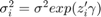
% Housekeeping
clear all
close all
clc

% Load Data set
load('data_harvey')

X = [ones(size(TableF61.LF,1),1),log(TableF61.Q),(log(TableF61.Q)).^2,log(TableF61.PF)];
Y = log(TableF61.C);
X_aux = TableF61.LF;
[beta_ols,sigma,e,se_ols,se_rob] = my_ols(Y,X);

stat = {'Constant';'log(Output)';'log(Output^2)';'log(Price Fuel)'};
t = table(stat,beta_ols,se_ols);
disp(t)

% Visual Inspection
figure(1)
hold on
grid on
plot(X_aux,e,'ko','MarkerFaceColor','k')
yline(0)
ylim([-0.4,0.4])
ylabel('Residual')
xlabel('Load Factor')
           stat            beta_ols     se_ols
    ___________________    ________    ________

    {'Constant'       }      9.1382     0.23956
    {'log(Output)'    }     0.92615     0.03158
    {'log(Output^2)'  }    0.029145    0.012027
    {'log(Price Fuel)'}     0.41006    0.018384
White Test
 Homoscedasticity
disp('White Test')
[value, pvalue] = my_white(e,X);
t = table(pvalue);
disp(t)
if pvalue<0.05
    disp('Reject Homoscedasticity')
else
    disp('Cannot Reject Homoscedasticity')
end
White Test
      pvalue
    __________

    4.4529e-05

Reject Homoscedasticity
LR test(Breusch Pagan)
Homoscedasticity
disp('BP test')
[result] = my_BP(e,X);
if result ==1
    disp('Reject Homoscedasticity')
else
    disp('Cannot Reject Homoscedasticity')
end
BP test
Reject Homoscedasticity
Estimate FGLS: Weighted
opt.het = 3;
[beta_fgls,~,se_fgls] = my_gls(Y,X,X_aux,opt);
stat = {'Constant';'log(Output)';'log(Output^2)';'log(Price Fuel)'};
t = table(stat,beta_ols,se_ols,se_rob,beta_fgls,se_fgls);
disp(t)

% Estimate FGLS: Inverse of the Variance
opt.het = 1;
[beta_fgls,~,se_fgls] = my_gls(Y,X,X_aux,opt);
stat = {'Constant';'log(Output)';'log(Output^2)';'log(Price Fuel)'};
t = table(stat,beta_ols,se_ols,se_rob,beta_fgls,se_fgls);
disp(t)
           stat            beta_ols     se_ols      se_rob     beta_fgls    se_fgls
    ___________________    ________    ________    ________    _________    ________

    {'Constant'       }      9.1382     0.23956     0.22595      9.2463      0.21404
    {'log(Output)'    }     0.92615     0.03158    0.030128     0.92136     0.032285
    {'log(Output^2)'  }    0.029145    0.012027    0.011346     0.02445     0.011155
    {'log(Price Fuel)'}     0.41006    0.018384    0.017524     0.40352     0.016592

           stat            beta_ols     se_ols      se_rob     beta_fgls     se_fgls
    ___________________    ________    ________    ________    _________    _________

    {'Constant'       }      9.1382     0.23956     0.22595      9.1335      0.032116
    {'log(Output)'    }     0.92615     0.03158    0.030128     0.92514     0.0054461
    {'log(Output^2)'  }    0.029145    0.012027    0.011346    0.028878     0.0020759
    {'log(Price Fuel)'}     0.41006    0.018384    0.017524     0.41027     0.0024223
Group Heteroscedasticity:
Example: Gasoline usage in 18 of the 30 OECD countries. The model analyzed is:

We suspect heteroscedasticity across countries (groups)
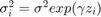
load('data_OECD')
par.nc = 18;% Number of countries
par.nt = 19;% Number of years

% Create Country dummy variables:
Xdum = zeros(par.nc*par.nt,par.nc);
for i = 1:par.nc
    if i ==1
        uv = i*par.nt;
        lv = uv-par.nt+1;
    else
        lv = uv+1;
        uv = i*par.nt;

    end
    Xdum(lv:uv,i) = 1;
end

Y = TableF91.LGASPCAR;
X = [TableF91.LINCOMEP,TableF91.LRPMG,TableF91.LCARPCAP,Xdum];

[beta_ols,sigma,e,se_ols,se_rob] = my_ols(Y,X);

stat = {'log(INC PC)';'log(PRICE)';'log(CAR PC)';'C1';'C2';'C3';'C4';...
    'C5';'C6';'C7';'C8';'C9';'C10';'C11';'C12';'C13';'C14';'C15';'C16';'C17';'C18'};
t = table(stat,beta_ols,se_ols);
disp(t)
         stat          beta_ols     se_ols
    _______________    ________    ________

    {'log(INC PC)'}     0.66225    0.071097
    {'log(PRICE)' }     -0.3217    0.042724
    {'log(CAR PC)'}    -0.64048    0.028753
    {'C1'         }      2.2859      0.2212
    {'C2'         }      2.1656     0.20626
    {'C3'         }      3.0418     0.21182
    {'C4'         }      2.3895      0.2016
    {'C5'         }      2.2048     0.20972
    {'C6'         }      2.1499     0.21109
    {'C7'         }      2.3371     0.20818
    {'C8'         }      2.5923     0.23609
    {'C9'         }      2.2325     0.23207
    {'C10'        }      2.3759     0.20523
    {'C11'        }      2.2348     0.20749
    {'C12'        }      2.2167     0.19671
    {'C13'        }      1.6818      0.1574
    {'C14'        }      3.0263     0.38221
    {'C15'        }      2.4025     0.22195
    {'C16'        }        2.51     0.22831
    {'C17'        }      2.3454      0.2202
    {'C18'        }      3.0553     0.21275
Visual Inspection
figure(2)
hold on
grid on
plot(TableF91.cn,e,'kx','linewidth',1.1)
yline(0)
ylabel('Residual')
xlabel('Country')
Then the weights are:

White Test
Homoscedasticity
disp('White Test')
[value, pvalue] = my_white(e,X);
%t = table(pvalue);
%disp(t)
if pvalue<0.05
    disp('Reject Homoscedasticity')
else
    disp('Cannot Reject Homoscedasticity')
end
White Test
Reject Homoscedasticity
LR test(Breusch Pagan)
Homoscedasticity
disp('BP test')
[result] = my_BP(e,X);
if result ==1
    disp('Reject Homoscedasticity')
else
    disp('Cannot Reject Homoscedasticity')
end
BP test
Reject Homoscedasticity
Estimate FGLS
opt.het = 0;
[beta_fgls,~,se_fgls] = my_gls(Y,X,[],opt,par);
t = table(stat,beta_ols,se_ols,se_rob,beta_fgls,se_fgls);
disp(t)
         stat          beta_ols     se_ols      se_rob     beta_fgls    se_fgls
    _______________    ________    ________    ________    _________    ________

    {'log(INC PC)'}     0.66225    0.071097    0.072774     0.57507     0.028354
    {'log(PRICE)' }     -0.3217    0.042724    0.053813    -0.27967     0.034088
    {'log(CAR PC)'}    -0.64048    0.028753    0.038761     -0.5654     0.015632
    {'C1'         }      2.2859      0.2212     0.22608      2.4371      0.10956
    {'C2'         }      2.1656     0.20626     0.20983       2.317     0.099057
    {'C3'         }      3.0418     0.21182     0.22479      3.2065      0.11299
    {'C4'         }      2.3895      0.2016     0.20783      2.5471     0.099305
    {'C5'         }      2.2048     0.20972     0.21087      2.3386     0.097857
    {'C6'         }      2.1499     0.21109     0.21846      2.3007      0.10553
    {'C7'         }      2.3371     0.20818     0.21801      2.5721      0.10856
    {'C8'         }      2.5923     0.23609      0.2347      2.7238      0.11029
    {'C9'         }      2.2325     0.23207     0.22973       2.348      0.10458
    {'C10'        }      2.3759     0.20523     0.22643      2.5899      0.11453
    {'C11'        }      2.2348     0.20749     0.21311      2.3962      0.10151
    {'C12'        }      2.2167     0.19671       0.203      2.3849     0.096395
    {'C13'        }      1.6818      0.1574     0.17133      1.9031     0.078924
    {'C14'        }      3.0263     0.38221      0.3918      3.0782       0.1977
    {'C15'        }      2.4025     0.22195      0.2328      2.5649      0.11524
    {'C16'        }        2.51     0.22831     0.26168      2.8235      0.12911
    {'C17'        }      2.3454      0.2202     0.22322      2.4821      0.10613
    {'C18'        }      3.0553     0.21275     0.22705      3.2152      0.11545
Estimate FGLS: Inverse variance weight
opt.het = 1;
[beta_fgls,~,se_fgls] = my_gls(Y,X,[],opt,par);
t = table(stat,beta_ols,se_ols,se_rob,beta_fgls,se_fgls);
disp(t)
         stat          beta_ols     se_ols      se_rob     beta_fgls     se_fgls
    _______________    ________    ________    ________    _________    _________

    {'log(INC PC)'}     0.66225    0.071097    0.072774     0.64884      0.010141
    {'log(PRICE)' }     -0.3217    0.042724    0.053813    -0.31172      0.005354
    {'log(CAR PC)'}    -0.64048    0.028753    0.038761     -0.6284     0.0056359
    {'C1'         }      2.2859      0.2212     0.22608      2.3286      0.029097
    {'C2'         }      2.1656     0.20626     0.20983      2.1946      0.025651
    {'C3'         }      3.0418     0.21182     0.22479      3.0753      0.027824
    {'C4'         }      2.3895      0.2016     0.20783      2.4175      0.025187
    {'C5'         }      2.2048     0.20972     0.21087      2.2311      0.025489
    {'C6'         }      2.1499     0.21109     0.21846      2.1824      0.027327
    {'C7'         }      2.3371     0.20818     0.21801      2.3819      0.027041
    {'C8'         }      2.5923     0.23609      0.2347      2.6286      0.029047
    {'C9'         }      2.2325     0.23207     0.22973      2.2587      0.028327
    {'C10'        }      2.3759     0.20523     0.22643      2.4207      0.027214
    {'C11'        }      2.2348     0.20749     0.21311      2.2657      0.025942
    {'C12'        }      2.2167     0.19671       0.203      2.2491      0.024314
    {'C13'        }      1.6818      0.1574     0.17133      1.7218      0.019432
    {'C14'        }      3.0263     0.38221      0.3918      3.0477      0.052502
    {'C15'        }      2.4025     0.22195      0.2328      2.4371      0.029051
    {'C16'        }        2.51     0.22831     0.26168       2.561      0.031624
    {'C17'        }      2.3454      0.2202     0.22322      2.3737      0.027897
    {'C18'        }      3.0553     0.21275     0.22705      3.0885      0.028447
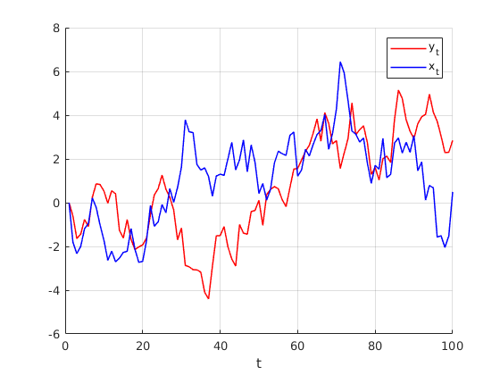
Activity 2: Spurious Relations
The case of non-stationaty series
Construct two independent random walk proceses


Where  and
and 
rng(123);
n = 100;
y = zeros(n,1);
x = zeros(n,1);
ey = randn(n,1);
ex = randn(n,1);

for i = 2:n
    y(i) = y(i-1) + ey(i);
    x(i) = x(i-1) + ex(i);
end

% Running Regression
[beta_ols,sigma,e,se_ols,se_rob] = my_ols(y,[ones(n,1),x]);

stat = {'beta'};
t = table(stat,beta_ols(2),se_ols(2));
disp(t)
      stat       Var2       Var3
    ________    _______    _______

    {'beta'}    0.34974    0.10816
Visual inspection
figure(3)
hold on
grid on
plot(1:n,y,'r-','linewidth',1.1)
plot(1:n,x,'b-','linewidth',1.1)
legend('y_{t}','x_{t}')
xlabel('t')
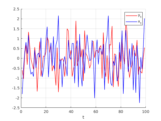
Detrending the variables
yd = y(2:end,1)-y(1:end-1,1);
xd = x(2:end,1)-x(1:end-1,1);
Visual inspection
figure(4)
hold on
grid on
plot(1:n-1,yd,'r-','linewidth',1.1)
plot(1:n-1,xd,'b-','linewidth',1.1)
legend('y_{t}','x_{t}')
xlabel('t')

% Running Regression
[beta_ols,sigma,e,se_ols,se_rob] = my_ols(yd,[ones(n-1,1),xd]);

stat = {'beta'};
t = table(stat,beta_ols(2),se_ols(2));
disp(t)
      stat        Var2        Var3
    ________    ________    ________

    {'beta'}    0.067435    0.084084
End of Code
dert_stop = 1;
%-------------------------------------------------
function [beta,e,se] = my_gls(y,x,x_aux,opt,par)
%{
This function computes GLS estimates and
its standard errors
inputs: y dependent var
        x independent vars
outputs: beta   OLS coefficients
         sigma  Estimator or variance of error
         e      Backed residuals
         se     Standard Errors
%}
    [n,k] = size(x);
    if opt.het==1
        % Tradicional heteroskedasticity
        [~,~,e_ols] = my_ols(y, x);
        e_ols = e_ols.^2;
        %C = diag(1./ sqrt(e_ols));
        C = chol(inv(diag(e_ols)));
        [beta,~,e,se] = my_ols(C*y, C*x);
    elseif opt.het==2
        % AR(1) Errors
        [~,~,e_ols] = my_ols(y, x);

        % estimation of AR(1) coefficient
        ey = e_ols(2:n);
        ex = e_ols(1:n-1);
        rho = ex\ey;            % Estimating the autocorrelation coeff
        e_auto = ey-ex*rho;
        var_e = var(e_auto);

        %factor = eye(n).*var_e./(1-rho^2);     % Cancels out
        sigma_e = eye(n);
        for i = 1:n
            for j = i+1:n
                sigma_e(i,j) = rho^(j-i);
                sigma_e(j,i) = sigma_e(i,j);
            end
        end
        %sigma_e = factor.*sigma_e;
        C = chol(inv(sigma_e));
        [beta,~,e,se] = my_ols(C*y, C*x);
    elseif opt.het==3
        % Weighted Least Squares:
        [~,~,e_ols] = my_ols(y, x);
        ye = log(e_ols.^2);
        xe = [ones(n,1),x_aux];
        [c,~,~,~] = my_ols(ye, xe);
        wgt = exp(-c(1)-c(2).*x_aux);
        [beta,~,e,se] = my_ols(y.*sqrt(wgt), x.*repmat(sqrt(wgt),1,k));
    else % By group
        % lets group the residuals
        [~,~,e_ols] = my_ols(y, x);
        e_aux = e_ols.^2;
        e_aux = reshape(e_aux,par.nt,par.nc);
        e_aux = mean(e_aux,1);
        e_aux = repmat(e_aux,par.nt,1);
        wgt = 1./e_aux(:);
        [beta,~,e,se] = my_ols(y.*sqrt(wgt), x.*repmat(sqrt(wgt),1,k));

    end % end if
end

%-------------------------------------------------------------------------
function [beta,sigma,e,se,se_rob] = my_ols(y,x)
%{
This function computes OLS estiamtes and
its standard errors
inputs: y dependent var
        x independent vars
outputs: beta   OLS coefficients
         sigma  Estimator or variance of error
         e      Backed residuals
         se     Standard Errors
%}
    [n,k] = size(x);
    beta = x\y;
    sigma = (y-x*beta)'*(y-x*beta)/(n-rank(x));
    e = y - x*beta;
    VCV = (e'*e)/n*inv(x'*x);
    se = sqrt(diag(VCV));

    % Eicker-White se
   aux = x.*(kron(e.^2,ones(1,k)));
	VCV_white = inv(x'*x) * x'*aux* inv(x'*x);


    se_rob = sqrt(diag(VCV_white));
end
%---------------------------------------------------------
function [value, pvalue] = my_white(e, x)
%{
 White's test for heteroscedasticity
 Input:
	e: Residuals
	x: Independent Variables
%}
	n = size(e,1);
	k = size(x,2) - 1;
	[~,~,e_ols] =my_ols(e.^2,x);
    TSS = e.^2 - mean(e.^2);
	TSS = TSS' * TSS;
	ESS = e_ols' * e_ols;
	rsq = 1 - ESS / TSS;  % the r-square auxiliary
	value = n*rsq;                  % Statistic
	pvalue = 1 - chi2cdf(value,k);  % Value
end

function [result] = my_BP(e, x)
%{
 Breusch pagan test for heteroscedasticity
 Input:
	e: Residuals
	x: Independent Variables
%}

	n = size(e,1);
	k = size(x,2);
	%[~,~,e_ols] =my_ols(e.^2,x);

    g = (e.^2)./((e'*e)./n)-1;
    LM = 0.5.*(g'*x*inv(x'*x)*x'*g);
    crit = chi2inv(0.95,k);
    if LM>crit
        result = 1; % Reject Ho
    else
        result = 0; % Cannot Reject H0
    end

end