Econometrics I
TA Christian Alemán
Session 8: Monday 14, March 2022
1: Measurement Error
- Measurement error in the dependent variable
- Measurement error in the independent variable
- IV Estimation
The case with no measurement error
Consider the following DGP:
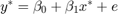

% Housekeeping
clear
clc
close all


% Set seed for reproductibility
rng(123)

N=1000;
betas = [2 2]';
err = sqrt(2).*randn(N,1);
x2_star = 10+2.*randn(N,1);
X_star = [ones(N,1) x2_star];
y_star = X_star*betas +err;
ols_func = @(X,y) (X'*X)\(X'*y);


% The OLS estimation of the true model is
names = str2mat("beta_{0}", "beta_{1}");

[b] = mc_ols(y_star, X_star, names, 0, 1);
y_pred = X_star*b;

figure(1)
hold on
plot(x2_star,y_star,'kx','MarkerFaceColor','k')
plot(x2_star, y_pred,'m-','linewidth',1.1)
ylabel('$y_{i}$', 'interpreter','latex')
xlabel('$x_{2,i}$','interpreter','latex')
title('No measurement error')
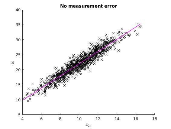
1.1: Measurement error in the dependent variable

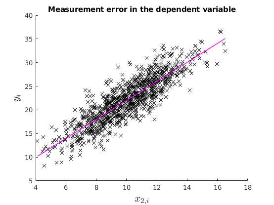
In this case OLS is still unbiased and consistent.
v =  2.*randn(N,1);
y = y_star +v;

% OLS estimation
[b] = mc_ols(y, X_star, names, 0, 1);
y_pred = X_star*b;

figure(2)
hold on
plot(x2_star,y,'kx','MarkerFaceColor','k')
plot(x2_star, y_pred,'m-','linewidth',1.1)
ylabel('$y_{i}$', 'interpreter','latex','fontsize',16)
xlabel('$x_{2,i}$','interpreter','latex','fontsize',16)
title('Measurement error in the dependent variable')

% See that with Montecarlo experiment:
no_reps = 1000;
K = size(X_star,2);
MC_betas = nan(no_reps,K);

 for i = 1:no_reps
    e_rep = sqrt(4).*randn(N,1);  %The error term of the regression
    y_star = X_star*betas +e_rep;
    v = 2.*randn(N,1);
    y_rep = y_star +v;
    MC_betas(i,:) = (ols_func(X_star,y_rep))';
 end

figure(3)
histfit(MC_betas(:,2))
xline(mean(MC_betas(:,2)),'k-','linewidth',1.2)
title('$\hat{beta}_{1}$','Interpreter','latex')
*********************************************************
OLS estimation results
Observations 1000
R-squared 0.745898
Sigma-squared 6.189020

Results (Ordinary var-cov estimator)

          estimate   st.err.   t-stat.   p-value
beta_{0}       1.897       0.381       4.984       0.000
beta_{1}       2.010       0.037      54.125       0.000

*********************************************************
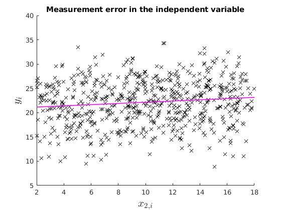
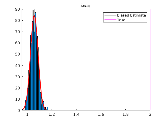
1.2: Measurement error in the explanatory variable: Attenuation bias
% 
Under attenuation bias then OLS estimator will be biased towards 0.
% Now suppose our dependent variable is measured with error
v =  8.*randn(N,1);
x2 = x2_star +v;

X = [ones(N,1) x2];

% OLS estimation
[b] = mc_ols(y_star, X, names, 0, 1);
y_pred = X*b;

figure(4)
hold on
plot(x2,y_star,'kx','MarkerFaceColor','k')
plot(x2, y_pred,'m-','linewidth',1.2)
ylabel('$y_{i}$', 'interpreter','latex','fontsize',16)
xlabel('$x_{2,i}$','interpreter','latex','fontsize',16)
xlim([2,18])
ylim([5,40])
title('Measurement error in the independent variable')

% See that with Montecarlo experiment:

K = size(X,2);
MC_betas = nan(no_reps,K);

 for i = 1:no_reps
    e_rep = sqrt(4).*randn(N,1);  %The error term of the regression
    y_star = X_star*betas +e_rep;
    v = 2.*randn(N,1);
    x2 = x2_star +v;       %Classical additive measurement error
    X = [ones(N,1) x2];
    MC_betas(i,:) = (ols_func(X,y_star))';
 end


figure(5)
hold on
histfit(MC_betas(:,2))
p1 = xline(mean(MC_betas(:,2)),'k-','linewidth',1.2);
p2 = xline(2,'m-','linewidth',1.2);
title('$\hat{beta}_{1}$','Interpreter','latex')
legend([p1,p2],{'Biased Estimate','True'})
*********************************************************
OLS estimation results
Observations 1000
R-squared 0.049470
Sigma-squared 21.048797

Results (Ordinary var-cov estimator)

          estimate   st.err.   t-stat.   p-value
beta_{0}      20.894       0.229      91.191       0.000
beta_{1}       0.125       0.017       7.207       0.000

*********************************************************
Dealing with measurement error
- IV
- 2SLS
Example Instrumental Variable Estimation.
n = 1000;

z1 = 3.*randn(n,1);
z2 = 2.*randn(n,1);

x = 3-2*z2+4*z1+randn(n,1);
y = 2+2*x +12*z2+randn(n,1);

% Case with no ommited variable

X = [ones(n,1) x z2];
names = str2mat("beta_{0}", "beta_{1}", "beta_{2}");
b = mc_ols(y, X, names, 0, 1);
*********************************************************
OLS estimation results
Observations 1000
R-squared 0.998771
Sigma-squared 0.998597

Results (Ordinary var-cov estimator)

          estimate   st.err.   t-stat.   p-value
beta_{0}       2.043       0.033      62.688       0.000
beta_{1}       2.001       0.003     770.861       0.000
beta_{2}      12.004       0.017     688.998       0.000

*********************************************************
Suppose we only observe x and z1:
Case with ommited variable:
X = [ones(n,1)  x];
names = str2mat("beta_{0}", "beta_{1}");
[b] = mc_ols(y, X, names, 0, 1);
*********************************************************
OLS estimation results
Observations 1000
R-squared 0.413590
Sigma-squared 475.999738

Results (Ordinary var-cov estimator)

          estimate   st.err.   t-stat.   p-value
beta_{0}       3.591       0.710       5.059       0.000
beta_{1}       1.423       0.054      26.531       0.000

*********************************************************
Solution
We can use z1 as an intrument:
- z1 is correlated with x
- z1 is not correlation to z2, thus not correlated with the residuals
Case 1: A very good instrument
disp('Check Correlation between x and z1')
disp(corr(x,z1))

Z = [ones(n,1) z1];

[b] = mc_olsIV(y,X,Z, names, 0, 1);
%b_IV= inv(Z'*X)*Z'*y
Check Correlation between x and z1
    0.9501


*********************************************************
OLS estimation results
Observations 1000
R-squared 0.354973
Sigma-squared 523.580490

Results (Ordinary var-cov estimator)

          estimate   st.err.   t-stat.   p-value
beta_{0}       1.920       0.724       2.652       0.008
beta_{1}       1.959       0.119      16.477       0.000

*********************************************************
Two Stage Least Squares
b_hat_x = inv(Z'*Z)*Z'*X;
X_hat = Z*b_hat_x;

[b] = mc_ols(y,X_hat, names, 0, 1);
%b_2SLS = inv(X_hat'*X_hat)*X_hat'*y
*********************************************************
OLS estimation results
Observations 1000
R-squared 0.707395
Sigma-squared 237.512636

Results (Ordinary var-cov estimator)

          estimate   st.err.   t-stat.   p-value
beta_{0}       1.920       0.503       3.818       0.000
beta_{1}       1.959       0.040      49.120       0.000

*********************************************************
Case 2: A good instrument
z1= 0.9.*randn(n,1);
x = 3- 2*z2+4*z1+randn(n,1);
y = 2+ 2*x +12*z2+randn(n,1);

disp('Check Correlation between x and z1')
disp(corr(x,z1))


X = [ones(n,1)  x];
Z = [ones(n,1) z1];

[b] = mc_olsIV(y,X,Z, names, 0, 1);
%b_IV= inv(Z'*X)*Z'*y
Check Correlation between x and z1
    0.6684


*********************************************************
OLS estimation results
Observations 1000
R-squared -0.859892
Sigma-squared 553.530829

Results (Ordinary var-cov estimator)

          estimate   st.err.   t-stat.   p-value
beta_{0}       1.339       0.748       1.791       0.074
beta_{1}       2.130       0.412       5.170       0.000

*********************************************************
Two Stage Least Squares
b_hat_x = inv(Z'*Z)*Z'*X;
X_hat = Z*b_hat_x;

[b] = mc_ols(y,X_hat, names, 0, 1);
%b_2SLS = inv(X_hat'*X_hat)*X_hat'*y


dert_stop = 1;
*********************************************************
OLS estimation results
Observations 1000
R-squared 0.194707
Sigma-squared 239.666920

Results (Ordinary var-cov estimator)

          estimate   st.err.   t-stat.   p-value
beta_{0}       1.339       0.645       2.076       0.038
beta_{1}       2.130       0.137      15.534       0.000

*********************************************************
Case 3: A weak instrument
z1= 0.07.*randn(n,1);
x = 3- 2*z2+4*z1+randn(n,1);
y = 2+ 2*x +12*z2+randn(n,1);

disp('Check Correlation between x and z1')
disp(corr(x,z1))


X = [ones(n,1)  x];
Z = [ones(n,1) z1];

[b] = mc_olsIV(y,X,Z, names, 0, 1);
%b_IV= inv(Z'*X)*Z'*y
Check Correlation between x and z1
    0.0707


*********************************************************
OLS estimation results
Observations 1000
R-squared -0.326477
Sigma-squared 319.804815

Results (Ordinary var-cov estimator)

          estimate   st.err.   t-stat.   p-value
beta_{0}       5.832       0.417      14.000       0.000
beta_{1}       0.632       4.026       0.157       0.875

*********************************************************
Two Stage Least Squares
b_hat_x = inv(Z'*Z)*Z'*X;
X_hat = Z*b_hat_x;

[b] = mc_ols(y,X_hat, names, 0, 1);
%b_2SLS = inv(X_hat'*X_hat)*X_hat'*y


dert_stop = 1;
Functions
%-------------------------------------------------------------

function [beta,sigma,r]= ols(y,x)
% Simple OLS regression
t = size(x,1);
beta = inv (x'*x) * x' * y;
sigma = (y-x*beta)'*(y-x*beta)/(t-rank(x));
r = y - x*beta;

end
%-------------------------------------------------------------


function prettyprint(mat, rlabels, clabels)
%{
This function prints matrices with row and column labels

Copyright (C) 2010 Michael Creel <michael.creel@uab.es>
This program is free software; you can redistribute it and/or modify
it under the terms of the GNU General Public License as published by
the Free Software Foundation
%}
	% left pad the column labels
	a = size(rlabels,2);
	for i = 1:a
		fprintf(' ');
	end
	fprintf('  ');

	% print the column labels
    try
	clabels = ['        ';clabels]; % pad to 8 characters wide
    catch
        dert_stop = 1;
    end
	clabels = strjust(clabels,'right');

	k = size(mat,2);
	for i = 1:k
		fprintf('%s  ',clabels(i+1,:));
	end

	% now print the row labels and rows
	fprintf('\n');
	k = size(mat,1);
	for i = 1:k
		if ischar(rlabels(i,:))
			fprintf(rlabels(i,:));
		else
			fprintf('%i', rlabels(i,:));
		end
		fprintf('  %10.3f', mat(i,:));
		fprintf('\n');
	end
end


function result = eemult_mv(m,v)

	if not(ismatrix(m))
		error("eemult_mv: first arg must be a matrix");
    end

	if not(isvector(v))
		error("eemult_mv: second arg must be a vector");
    end

	[rm, cm] = size(m);
	[rv, cv] = size(v);

	if (rm == rv)
		v = kron(v, ones(1,cm));
		result = m .* v;
	elseif (cm == cv)
		v = kron(v, ones(rm, 1));
		result = m .* v;
	else
		error("eemult_mv: dimension of vector must match one of the dimensions of the matrix");
    end
end
%-------------------------------------------------------------

function [b, varb, e, ess] = mc_ols(y, x, names, silent, regularvc)
%{

Copyright (C) 2010 Michael Creel <michael.creel@uab.es>
This program is free software; you can redistribute it and/or modify
it under the terms of the GNU General Public License as published by
the Free Software Foundation

Calculates ordinary LS estimator using the Huber-White heteroscedastic
consistent variance estimator.

 inputs:
 y: dep variable
 x: matrix of regressors
 names (optional) names of regressors
 silent (bool) default false. controls screen output
 regularvc (bool) default false. use normal varcov estimator, instead of het consistent (default)

 outputs:
 b: estimated coefficients
 varb: estimated covariance matrix of coefficients (Huber-White by default, ordinary OLS if requested with switch)
 e: ols residuals
 ess: sum of squared residuals

%}
	k = size(x,2);

	if nargin < 5 regularvc = 0; end
	if nargin < 4 silent = 0; end
	if (nargin < 3) || (size(names,1) ~= k)
		names = 1:k;
		names = names';
	end

	[b, sigsq, e] = ols(y,x);


	xx_inv = inv(x'*x);
	n = size(x,1);

	ess = e' * e;

	% Ordinary or het. consistent variance estimate
	if regularvc==1
		varb = xx_inv*sigsq;
    end

	seb = sqrt(diag(varb));
	t = b ./ seb;

	tss = y - mean(y);
	tss = tss' * tss;
	rsq = 1 - ess / tss;

	labels = char('estimate', 'st.err.', 't-stat.', 'p-value');
	if silent==0
		fprintf('\n*********************************************************\n');
		fprintf('OLS estimation results\n');
		fprintf('Observations %d\n',n);
		fprintf('R-squared %f\n',rsq);
		fprintf('Sigma-squared %f\n',sigsq);
		p = 2 - 2*tcdf(abs(t), n - k);
		results = [b, seb, t, p];
		if regularvc
			fprintf('\nResults (Ordinary var-cov estimator)\n\n');
		else
			fprintf('\nResults (Het. consistent var-cov estimator)\n\n');
		end
		prettyprint(results, names, labels);
		fprintf('\n*********************************************************\n');
	end

end
%-------------------------------------------------------------

function [b, varb, e, ess] = mc_olsIV(y, x, z, names, silent, regularvc)
%{

Copyright (C) 2010 Michael Creel <michael.creel@uab.es>
This program is free software; you can redistribute it and/or modify
it under the terms of the GNU General Public License as published by
the Free Software Foundation

Calculates ordinary LS estimator using the Huber-White heteroscedastic
consistent variance estimator.

 inputs:
 y: dep variable
 x: matrix of regressors
 names (optional) names of regressors
 silent (bool) default false. controls screen output
 regularvc (bool) default false. use normal varcov estimator, instead of het consistent (default)

 outputs:
 b: estimated coefficients
 varb: estimated covariance matrix of coefficients (Huber-White by default, ordinary OLS if requested with switch)
 e: ols residuals
 ess: sum of squared residuals

%}
	k = size(x,2);

	if nargin < 6 regularvc = 0; end
	if nargin < 5 silent = 0; end
	if (nargin < 4) || (size(names,1) ~= k)
		names = 1:k;
		names = names';
	end

	%[b, sigsq, e] = ols(y,x);
    t = size(x,1);
    b = inv(z'*x)*z'*y;
    sigsq = (y-x*b)'*(y-x*b)/(t-rank(x));
    e = y - x*b;


	xx_inv = inv(z'*x);
	n = size(x,1);

	ess = e' * e;

	% Ordinary or het. consistent variance estimate
	if regularvc==1
		varb = xx_inv*sigsq;
	end

	seb = sqrt(diag(varb));
	t = b ./ seb;

	tss = y - mean(y);
	tss = tss' * tss;
	rsq = 1 - ess / tss;

	labels = char('estimate', 'st.err.', 't-stat.', 'p-value');
	if silent==0
		fprintf('\n*********************************************************\n');
		fprintf('OLS estimation results\n');
		fprintf('Observations %d\n',n);
		fprintf('R-squared %f\n',rsq);
		fprintf('Sigma-squared %f\n',sigsq);
		p = 2 - 2*tcdf(abs(t), n - k);
		results = [b, seb, t, p];
		if regularvc
			fprintf('\nResults (Ordinary var-cov estimator)\n\n');
		else
			fprintf('\nResults (Het. consistent var-cov estimator)\n\n');
		end
		prettyprint(results, names, labels);
		fprintf('\n*********************************************************\n');
	end

end
*********************************************************
OLS estimation results
Observations 1000
R-squared 0.904879
Sigma-squared 1.961686

Results (Ordinary var-cov estimator)

          estimate   st.err.   t-stat.   p-value
beta_{0}       1.621       0.214       7.566       0.000
beta_{1}       2.038       0.021      97.437       0.000

*********************************************************